Fano Varieties and Extremal Laurent Polynomials

Statistics

July 7, 2011, 1:45 pm

Notations:
p.s. – period sequence
fano p.s. – one of 105 p.s. of smooth Fano 3-folds
good p.s. – p.s. s.t. P_0(D) has integer roots, where L = sum_{i=0}^r t^i P_i(D) is the diff.op. annihilating p.s.
bad p.s. – not good p.s.

LP – Laurent polynomial.
fano LP – Laurent polynomial for which RG coincides with one of 105 fano p.s.

Everywhere below we put a binomial condition (of Coates-Corti-Galkin-Golyshev-Przjyalkowski-Usnich-etc) on the edges.

MP – Minkowski Laurent polynomial
PP – (Coates-)Przyjalkowski Laurent polynomial (binomial on edges, zero everywhere else)

This is the statistics of reflexive 3-polytopes.

—

18 are smooth.

—

100 (= 18+82) are terminal. They give rise to 100 LP and 62 good p.s.

—

899 (= 18+82+799) has no integer points in interior of facets.

Each one gives rise to a unique MP (which coincides with PP).

712 of these MPs are fano LP – they give rise to 92 fano p.s.
187 are bad – they give rise to 63 bad p.s.

92 = 98-6, where 98 = 105-7.
The 7 that didn’t appear among MP p.s.’s are:
V_2 [bottom degree],
its double cover B_1 [bottom degree in rho=1, r=2],
2.1, 2.2, 2.3 [bottom degree in rho=2],
P^1 x S_2, P^1 x S_1 [top Picard rank].

The extra 6 Fano (p.s.) that didn’t appear are:
V_4 (15), V_6 (19), V_8 (5), V_{10} (9), V_{12} (7) [next bottom degree in rho=1,r=1);
2.4 (49) [next bottom degree in rho=2].

So they lie at the bottom of the list, just over the non-appearing 5.

—

1051 polytopes has exactly one integer point in the respective interior of the facets (i.e. not origin, vertex, and not on the edge).

The facet that contains the extra integer point is then on of famous 16 reflexive 2-polytopes,
so 1051 polytopes fall into 16 classes.

Number of polytopes in each class is as follows (total 1051):
[20, 24, 125, 50, 75, 196, 22, 86, 111, 74, 64, 112, 19, 42, 23, 8]

Number of fano LP in each class is as follows (total 1055):
[0, 20, 0, 47, 61, 187, 27, 123, 195, 140, 56, 109, 17, 42, 23, 8]
which is
[0,17+3,0,44+3,61,187,16+11,71+52,107+88,70+70,56,109,17,42,23,8]

Our enumeration and “fano” values for the extra coefficient are as follows:

number – associated vertex Laurent polynomial – class – #poly – values [number of appearances]

0 – x+y+1/x/y – P^2 – 20 – nothing
1 – y + x/y + 1/x/y – Q – 24 – 0 [17], 4 [3]
2 – x+y+xy+1/x/y – S_8 – 125 – nothing
3 – x+y+1/x+1/y – Q – 50 – 0 [44], 4 [3]
4 – y+x+x/y+1/x/y – S_7 – 75 – 1 [61]
5 – x+y+1/x+1/y+xy – S_7 – 196 – 1 [187]
6 – y/x+1/x/y+x^2/y – S_6 – 22 – 2 [16], 3 [11]
7 – y+y/x+1/x/y+x/y – S_6 – 86 – 2 [71], 3 [52]
8 – y+x+1/x+x/y+1/x/y – S_6 – 111 – 2 [107], 3 [88]
9 – x+y+x/y+1/x+1/y+y/x – S_6 – 74 – 2 [70], 3 [70]
10- x+y/x+1/x/y+x^2/y – S_5 – 64 – 3 [56]
11- x+y+y/x+x/y+1/x+1/y+1/x/y – S_5 – 112 – 3 [109]
12- y+x+1/x+x^2/y+1/x^2/y – S_4 – 19 – 4 [17]
13- y+y/x+1/x/y+x^2/y – S_4 – 42 – 4 [42]
14- xy+y/x+x/y+1/x/y – S_4 – 23 – 4 [23]
15- 1/x/y+x^2/y+y^2/x – S_3 – 8 – 6 [8]

Of course everything is extremal and Hodge-Tate,
but some are not-Minkowski, and not even SCR-equivalent (using only surface mutations of the respective facet) to any Minkowski
(in particular examples with class Q and coefficient a=4,
also those in Q with coeff a=0 are not lattice Minkowski, but Minkowski).
1-puzzles

Posted by: Sergey Galkin | 1 Comment

It’s all gone frighteningly meta

June 30, 2011, 10:02 pm

I’m speaking about the Fanosearch project at the Social Media and the Academy conference at UCL tomorrow. Slides are here; handout is here.

Posted by: Tom | Comment

Logistics update

June 11, 2011, 9:15 pm

A quick update on the 4-dimensional calculation. Right now we are calculating basic data (faces, degree, Hilbert series, integer points, smooth/terminal/canonical, etc.) for all the 4d reflexive polytopes in the Kreuzer–Skarke list. The current computational setup is: one central database server for distributing parts of the calculation, storing results, etc, and a number of “worker nodes”, which are jobs running on the Imperial Maths computer cluster. The worker nodes are where the calculations are actually done.

Initially we were running with around 30 worker nodes, and the rate of progress suggested that the calculation would finish in about 4 years. This looked encouraging, as we will in the end use a much larger number of worker nodes (several hundred). But recently we have been running with more workers (60-80) and the calculation has slowed down considerably: at current rate it will finish in around 40 years. This seems strange, as we are now throwing more computer power at the problem.

Al has discovered that the bottleneck is not the calculations themselves, but database locking. Since we need to check as part of our calculation that every polytope occurs only once in the list, only one worker may write to the results database at once. Thus it needs to get a lock on the results database before it writes to it, and frees that lock after it has finished writing data. Also there are several locking steps, with both read and write locks, in the code which distributes jobs to workers. Workers are spending a huge fraction of their time waiting for database locks, and it is this that is slowing the computation down.

Al has had a clever idea about how to fix this, which should significantly decrease the locking overhead. Also we will move the databases which keep track of locks off Fano (the main database server) and onto their own dedicated machines; this should help a lot too. We will update here (and tweet) once we have a good idea of how the new code performs. Hopefully it will scale well, as the next steps involve managing calculations across many more computers.

Future:

more workers, running on the Imperial College HPC (High Performance Computing) service. This should be quick and easy to get going, a matter of a couple of weeks.
more workers, running on SCAN (the Imperial Supercomputer At Night, which is ~200 PCs in the Maths department. This will take longer to set up, as the SCAN runs FreeBSD and so we need to get our worker nodes running under FreeBSD. The Magma team are working on a FreeBSD build of Magma (hooray!) but this is a new platform for them and so we will need to do some careful testing.
the next steps in the 4d calculation. As soon as the locking issues are sorted out we should make a detailed plan for the next two or three months of calculations.

Posted by: Tom | Comment

Planning the 3-dimensional calculation

May 25, 2011, 1:25 pm

Al Kasprzyk, coding hero, has now more-or-less finished the parallel computation infrastructure. So now we should think about how to organize the 3d calculation. What should we compute, and in what order?

all Przyjalkowski polynomials supported on 3d reflexive polytopes, and their periods
all Minkowski decompositions of facets of 3d reflexive polytopes
all Minkowski polynomials supported on 3d reflexive polytopes, and their periods
Picard-Fuchs operators for Przyjalkowski and Minkowski period sequences
local monodromy data
what else? Please add to and modify this list.

Przyjalkowski polynomials = binomial coefficients along edges and zeroes everywhere else.

Posted by: Tom | Comment

Surface mutations

March 21, 2011, 6:48 am

I wrote a pari/gp script to do all the mutations in dimension 2 –
can mutate mirrors for all 10 del Pezzo surfaces.
By the way I found some typos (related to signs) in our paper.
See the file with the script for the correct formulas.

degmir.gp

Tags: code, mutations
Posted by: Sergey Galkin | Comment

Installing Python modules for Sage

March 4, 2011, 4:40 pm

This is more of a note to myself, but:
sage -python -m easy_install foo
will use easy_install (from Python setuptools) to install the python module foo in the correct place for Sage to find it.

Posted by: Tom | Comment

Quantum Lefshetz for non-split bundle via “abelian/non-abelian correspondence”.

February 15, 2011, 5:09 pm

Bumsig Kim explained me how their beautiful theory provides a tool for computing J-series of $V_{22}$ and many other Fano threefolds.

The computation for $V_{22}$ can be reproduced by the following pari/gp code (I omit checking that mirror map is almost trivial):

N=9 o = O(t^(N+1)) h(n) = sum(k=1,n,1/k) hh(n) = sum(k=1,n,sum(l=k+1,n,1/k/l)) gg(x, p) = (x!*(1+h(x)*p+hh(x)*p^2+O(u^4))) simplemirrormap(F) = F * exp(-polcoeff(F,1,t)*t) reg(F) = sum(n=0,N,t^n*polcoeff(F,n,t)*n!)+O(t^(N+1)) period(F) = reg(simplemirrormap(F))


gp > v22 = period( polcoeff( sum(a=0,N,sum(b=0,N,sum(c=0,N,o+ t^(a+b+c)* ( gg(a+b,u*(A+B)) * gg(a+c,u*(A+C)) * gg(b+c,u*(B+C)) )^3 / (gg(a,u*A) * gg(b,u*B) * gg(c,u*C) )^7 *(c-b+u*(C-B))*(c-a+u*(C-A))*(b-a+u*(B-A)) ))) + O(u^4) , 3,u) /(C-B)/(C-A)/(B-A) + o )

%2 = 1 + 12*t^2 + 60*t^3 + 636*t^4 + 5760*t^5 + 58620*t^6 + 604800*t^7 + 6447420*t^8 + O(t^9)
Indeed, period sequence 17.
Note that $gg(x,p) = \frac{\Gamma(1 + x + \frac{p}{z})}{\Gamma(1 + \frac{p}{z})} + o(\frac{1}{z^3})$ is the familiar Gamma-factor with $u=\frac{1}{z}$ .

——————————————————-

So, how does it works?

Consider 3-dimensional vector space $U = \CC^3$ with a fixed base, 7-dimensional vector space $V = \CC^7$ , and space $M = \CC^{21}$ of 3×7 matrices $M = Hom(U,V) =Hom(\CC^3, \CC^7)$

Group $G = Aut(U) = GL(3)$ acts on M by left multiplication. It has a subgroup $T = (\CC^*)^3$ of diagonal matrices and one may restrict the action to this smaller subgroup.

Let $M_{na}$ be the subset of matrices of maximal rank and $M_{ab}$ be the subset of matrices with non-vanishing rows, $M_{na}$ is an open subset in $M_{ab}$ .

Consider quotient spaces $X_{na} = M_{na} / G$ and $X_{ab} = M_{ab} / T$ . Note that $X_{na} = Gr(3,V) = Gr(3,7)$ and $X_{ab} = (\PP(V))^3 = (\PP^6)^3$ .

Since T is a subgroup of G, there is a natural rational map $\pi: X_{ab} -> X_{na}$ : a triple of points in $\PP^6$ is sent to their linear span.

Weyl group (symmetric group $S_3$ ) acts on $X_{ab} = (\PP^6)^3$ and hence it acts on the cohomology $H(X_{ab}) = H((\PP^6)^3)$ , so cohomology space is decomposed into representations of $S_3$ .

[I’ll omit the part of the story with the partial flag space and non-holomorphic map].

1. It turns out that cohomology $H(X_{na})$ can be identified with antisymmetric part of $H(X_{ab})$ as a graded vector space (with grading shifted by 3).
Explicitly, $H(X_{ab})$ is generated by 3 pullbacks $H_1, H_2, H_3$ of hyperplane sections on $\PP^6$ ; cohomologies of Grassmanian are known to be quotient of symmetric polynomials. Vector space of anti-symmetric polynomials is obtained from vector space of symmetric polynomials via multiplication by anti-symmetric polynomial of the smallest degree $Formula does not parse: \Delta = \prod_{i<j} (s_i-s_j)[/latex]. So cohomology class in Grassmanian corresponding to symmetric function [latex]\sigma[/latex] is sent into [latex]\Delta \cup \sigma(H_1,H_2,H_3)[/latex]. <b>2.</b>Also we can compare vector bundles on [latex]X_{ab}$ and $X_{na}$ by pulling them back to M, and considering as G-linearized.
It turns out that universal bundle U over Gr(3,7) decomposes into sum of 3 line bundles on $X_{ab}: U <-> O(1,0,0) \oplus O(0,1,0) \oplus O(0,0,1)$ .
So $O_{Gr(3,7)}(1) <-> O(1,1,1)$ and $U^*(1) <-> O(1,1,0) \oplus O(1,0,1) \oplus O(0,1,1)$ .

3. On domain of $\pi$ one may define a relative tangent bundle $T_{\pi}$ (“traceless” part of $Hom(U,U)$ ). It turns out this vector bundle can be extended as a split vector bundle to whole $X_{ab}$ : $T_{\pi} = O(1,-1,0) \oplus O(-1,1,0) \oplus O(1,0,-1) \oplus O(-1,0,1) \oplus O(0,1,-1) \oplus O(0,-1,1)$ .
Consider “square root” of relative tangent bundle $t_{\pi} = O(0,-1,1) \oplus O(-1,0,1) \oplus O(-1,1,0)$ .

4.Recall that Fano threefolds $V_{22} = V_{na}$ are sections of homogeneous vector bundle $E = 3 U^*(1)$ on $Gr(3,7)$ . Comparision (2) shows these threefolds has 9-dimensional abelianizations $V_{ab}$ — complete intersections of $9$-dimensional split bundle $E_{ab} = (O \oplus O \oplus O) \otimes (O(1,1,0) \oplus O(1,0,1) \oplus O(0,1,1))$ on $X_{ab}$ .

5. Abelian/non-abelian correspondence is similar for pairs $X_{ab}/X_{na}$ and $V_{ab}/V_{na}$ .
J-series for Gr(3,7) can be obtained as twisted by relative tangent bundle $T_{\pi}$ I-series for $e(t_{\pi}) \cup I_{X_{ab},T_{\pi}}$ after the comparision of cohomologies described in (1).
Similarly, J-series for $V_{22}$ can be obtained via mirror map from twisted by $T_{\pi} + E_{ab}$ I-series $e(t_{\pi}) \cup I_{X_{ab},T_{\pi}+E}$ after the “pullbacked” comparision (1).

6. The sign comes from considering closely the Gamma-factor for relative tangent bundle $T_{\pi}$ . Note that fibers of abelian/non-abelian correspondence are in some sense holomorphic symplectic (relative tangent bundle contains both O(D) and O(-D)), so they behave like varieties with trivial canonical class.
Consider the factor $\frac{\Gamma(1+D+d) \Gamma(1-D-d)}{\Gamma(1+D)\Gamma(1-D)}$ . Since $\Gamma(1+x) \Gamma(1-x) = \frac{\pi x}{sin (\pi x)}$ and $sin (\pi (x+d)) = (-1)^d sin(\pi x)$ we have $\frac{\Gamma(1+D+d) \Gamma(1-D-d)}{\Gamma(1+D)\Gamma(1-D)} = (-1)^d \frac{d+D}{D}$ .

The same method can also be applied to complete intersections of homogeneous bundles in orthogonal isotropic and symplectic isotropic Grassmanians, since these Grassmanians themselves are just sections of some homogeneous bundles (wedge or symmetric powers of universal bundle) on ordinary Grassmanians of type A. Also this can be uprgaded to treat different blowups of these varieties. In particular, in the comments to this post I compute J-series for Fano threefolds $V_5$ , #2.14, #2.17, #2.20, #2.21 and #2.22.

Also Bumsig points out that one can express the ab/non-ab twist as a differential operator applied to abelian multi-parameter J-function (basically, just Vandermonde $\prod_{i>j} (\frac{d}{d q_i} - \frac{d}{d q_j})$ . This interpretation is more useful for dealing with Frobenius manifolds.

References:
Gromov-Witten Invariants for Abelian and Nonabelian Quotients by Aaron Bertram, Ionut Ciocan-Fontanine, Bumsig Kim
The Abelian/Nonabelian Correspondence and Frobenius Manifolds by Ionut Ciocan-Fontanine, Bumsig Kim, Claude Sabbah
Quantum cohomology of the Grassmannian and alternate Thom-Sebastiani by Bumsig Kim, Claude Sabbah

Tags: code, example, geometry, theory
Posted by: Sergey Galkin | 3 Comments

Press release: animations

February 9, 2011, 10:24 pm

Below are animations showing some of the shapes that we have analyzed in our project so far. Please email me if you need higher or lower resolution versions. An explanation of what the animations show is here.

Animation 1: slices of the Fano variety $V_2$ seen from several different angles. Hi-res version. Low-res version.
Animation 2: slices of the Fano variety $V_4$ seen from two different angles. Hi-res version. Low-res version.
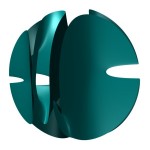
Animation 3: the cubic threefold, seen from the outside from various angles. Hi-res version.
Animation 4: the cubic threefold and slices through it. Hi-res version. Low-res version.
Animation 5: breaking up a shape into simpler pieces. This animation shows how a surface called a hyperboloid (the curved cylinder) is made up from straight lines (shown in red). You can think of the hyperboloid as a “molecule”, made up from “atoms” that are the straight lines. Hi-res version. Low-res version.

Posted by: Tom | 21,281 Comments

Press release: images

February 9, 2011, 9:57 pm

Below are images of some of the shapes that we have analyzed in our project so far. Clicking on any of the thumbnails leads to a larger version of the same image (at a resolution of 300dpi). Please email me if you need larger or higher-resolution images. A description of what the images show is here.

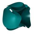
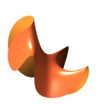
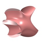
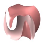
		slices of the Fano variety $V_6$
		slices of the cubic threefold
		slices of a Fano variety (#1 on the rank-2 list)
		slices of a Fano variety (#4 on the rank-2 list)
		slices of a Fano variety (#2 on the rank-4 list)
		slices of the quadric threefold
		slices of a Fano variety (#2 on the rank-2 list)
		slices of a Fano variety (#9 on the rank-3 list)

What are these images?

We are searching for special shapes, called Fano varieties, that are the “elements” in our “periodic table of shapes”. We created the images above when analyzing 3-dimensional Fano varieties. It is difficult to visualize a complex 3-dimensional shape, but one way to do it is to look at slices through the shape. For example, to visualize the human brain (which is also a complex 3-dimensional shape!) you can take slices using an MRI scanner, and then assemble these slices to view the whole brain, like this: (Thanks to Dr Daniel Bulte at the University of Oxford for the animation.)

The images above are slices of some of our Fano varieties. Our slices are curved surfaces (unlike the slices of brain, which are flat) because the Fano varieties themselves are curved 3-dimensional shapes: the slices become flat if you view them in four dimensions.

If you think of the fourth dimension as time, then a curved three-dimensional space becomes a family of surfaces (the slices pictured above) that change with time. To visualize the whole Fano variety this way, we created animations showing how these slices change with time.

Posted by: Tom | 1 Comment

A riddle wrapped in a mystery inside a balls-up

December 31, 2010, 11:43 am

Consider #2 on the Mori-Mukai list of rank-3 Fano 3-folds. This has been giving us some difficulty, which I have now resolved. We were making a combination of mistakes. Mori and Mukai describe the variety $X$ as follows.

A member of $|L^{\otimes 2} \otimes_{\cO_{\PP^1 \times \PP^1}} \cO(2,3)|$ on the $\PP^2$ -bundle $\PP(\cO \oplus \cO(-1,-1)^{\oplus 2})$ over $\PP^1 \times \PP^1$ such that $X \cap Y$ is irreducible, where $L$ is the tautological line bundle and $Y$ is a member of $|L|$ .

Our first mistake, as Mukai-sensei pointed out in an email to Corti, was using the wrong weight convention for projective bundles. Mori and Mukai use negative weights, so the ambient $\PP^2$ -bundle $F$ is the toric variety with weight data:
$\begin{array}{cccccccc} x_0 & x_1 & y_0 & y_1 & t_0 & t_1 & t_2 & \\ 1 & 1 & 0 & 0 & 0 & 1 & 1 & \\ 0& 0 & 1 & 1 & 0 & 1 & 1 & \\ 0 & 0 & 0 & 0& 1 &1 & 1 & \end{array}$
For later convenience we change basis, expressing $F$ as the toric variety with weight data:
$\begin{array}{cccccccc} x_0 & x_1 & y_0 & y_1 & t_0 & t_1 & t_2 & \\ 1 & 1 & 0 & 0 & -1 & 0 & 0 & A \\ 0& 0 & 1 & 1 & -1 & 0 & 0 & B \\ 0 & 0 & 0 & 0& 1 &1 & 1 & C \end{array}$
$X$ is a section of $|B+2C|$ .

Our second mistake was failing to accurately account for the fact that although $X$ is Fano, the bundle $A+C$ (which restricts to $-K_X$ on $X$ ) is only semi-positive on $F$ . Thus we are in the situation described in this post and, in the notation defined there, we have:
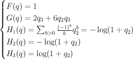
$\begin{cases} F(q) = 1 \\ G(q) = 2q_3+6q_2 q_3 \\ H_1(q) = \sum_{b>0} {(-1)^{b} \over b} q_2^b = {-\log(1+q_2)} \\ H_2(q) = {-\log(1+q_2)} \\ H_3(q) = \log(1+q_2) \end{cases}$
and hence:
$\begin{cases} q_1 = {\hat{q}_1 \over 1 - \hat{q}_2} \\ q_2 = {\hat{q_2} \over 1 - \hat{q_2}} \\ q_3 = \hat{q}_3 (1-\hat{q_2}) \end{cases}$
Thus the cohomological-degree-zero part of the J-function is:
$\exp({-2}\hat{q}_3(1-\hat{q}_2)-6\hat{q}_2 \hat{q}_3) \sum_{a,b,c\geq 0} \hat{q}_1^a \hat{q}_2^b \hat{q}_3^c(1-\hat{q}_2)^{c-b-a} {1 \over z^{a+c}} {(b+2c)! \over a!a!b!b!c!c!(c-b-a)!}$
and setting $\hat{q}_1 = t$ , $\hat{q}_2 = 1$ , $\hat{q}_3 = t$ , $z=1$ yields:
$\exp(-6t) \sum_{a,b\geq 0} t^{2a+b} {(2a+3b)! \over a!a!b!b!(a+b)!(a+b)!}$
Regularizing this gives:
$I_{reg}(t) =1+58 t^2+600 t^3+13182 t^4+247440 t^5+5212300 t^6+111835920 t^7+ \cdots$
As Galkin conjectured, this is period sequence 97.